Analyzing Landsat Image Metadata with the Spatial DataFrame

A guest post by Gregory Brunner

A few weeks ago, Esri released an update to the ArcGIS API for Python. The newest release includes:

• An intuitive and powerful raster API
• Powerful GIS administration
• Spatial DataFrames!!!

Hopefully, you can tell that the new functionality in the API that I am most excited about is the [spatial dataframe](http://developers.arcgis.com/help doc)! The spatial dataframe extends the pandas dataframe by adding geometry, spatial reference, and other spatial components to the dataframe. In adding the spatial dataframe to the API, ArcGIS users can now read feature classes, feature services, and image services directly into a dataframe. Once in a spatial dataframe, users can perform fast statistical and spatial analysis on the data, update existing feature services, and convert the dataframe to a feature class or shapefile. These are just a few examples of how you can use the spatial dataframe.

What really interests me is how this can be used with an ArcGIS image service. Can I use the spatial dataframe to extract image footprints from an image service? Can I use it to perform statistical analysis image footprints over a specific part of the world?

The answer to both of these questions is Yes! In this post, I’ll walk through how to use the API for Python to extract image service footprints from the Landsat 8 Views image service, show how to use a spatial filter to extract only footprints over New Jersey, determine the mean cloud cover and most recent acquisition date of the images, and share those image footprints as a feature service. If you have ever been interested in doing any of these, keep reading!

Getting Started

When using the ArcGIS API for Python, we first need to import the GIS.

import arcgis
from arcgis.gis import GIS
from IPython.display import display

# create a Web GIS object
gis = GIS("https://www.arcgis.com", "gregb")

We are going to look at Landsat footprints over the United States, so using gis.map we can open up our map over the USA.

#Looking over the USA
map1 = gis.map("USA", zoomlevel = 4)
display(map1)

Using search I can find the Landsat 8 Views service in ArcGIS.com and add that layer to the map.

landsat_search = gis.content.search('"Landsat 8 Views"',outside_org=True)
map1.add_layer(landsat_search[0])

I also need to grab the URL for this service and assign it to a variable.

url = landsat_search[0].url 
print(url)

https://landsat2.arcgis.com/arcgis/rest/services/Landsat8_Views/ImageServer

I am going to read the Landsat 8 Views service into a spatial dataframe. In order to do so, I will import SpatialDataFrame and ImageryLayer from arcgis.

from arcgis import SpatialDataFrame
from arcgis.raster._layer import ImageryLayer

Using ImageryLayer I will create the image service object.

imserv = ImageryLayer(url=url)

Within the image service object is a spatial dataframe. I can access it as follows.

image_service_sdf = imserv.query().df

I did not submit any query parameters here. I will do that shortly to show how you can specify query parameters such as a spatial filter.

The dataframe is essentially the attribute table.

image_service_sdf.head()

Let’s see how many footprints are in the dataframe.

print("There are " + str(len(image_service_sdf)) + " Landsat image service footprints in this dataframe.")

There are 1000 Landsat image service footprints in this dataframe.

There are 1000 Landsat image footprints in this dataframe. There are really hundreds of thousands, if not millions of images in this service. Only 1000 are returned because the service has a Max Record Count that is set to 1000.

Applying Query Parameters

Now that I know how to get the image service table as a spatial dataframe, I will apply a spatial filter so that I only retrieve image service footprints over New Jersey. I will also specify a where clause so that I only retrieve Primary footprints, meaning that I will exclude any Overview footprints from the dataframe.

In order to specify my extent, I am going to use arcpy and the Describe method to read a feature class that holds the geometry for New Jersey.

import arcpy

fc = r'C:\PROJECTS\STATE_OF_THE_DATA\DATA\usa_states\usa.gdb\nj'

grid_desc = arcpy.Describe(fc)
grid_sr = grid_desc.spatialReference
grid_extent = grid_desc.extent

In order to use this extent as a spatial filter on my image service query, I need to import filters from the ArcGIS API for Python.

from arcgis.geometry import filters

To create my filter, I need to pass the filter the geometry, the spatial reference, and the spatial relationship that I want the extent and the image service to have. In this case, I want to return footprints that intersect with New Jersey.

geometry = grid_extent
sr = grid_sr
sp_rel = "esriSpatialRelIntersects"
sp_filter = filters._filter(geometry, sr, sp_rel)

I also only want to return Primary image service footprints, meaning that I want to exclude the image service Overviews. I can do this by querying the Category field in the image service attribute table for footprints that have a value of 1.

search_field = 'Category'
search_val = 1
where_clause = search_field + '=' + str(search_val)

Now, when I query the image service and return the dataframe, I will also submit the where_clause and sp_filter. This should return only Primary image service footprints over New Jersey.

image_service_sdf = imserv.query(where=where_clause,geometry_filter=sp_filter,return_geometry=True).df
image_service_sdf.head()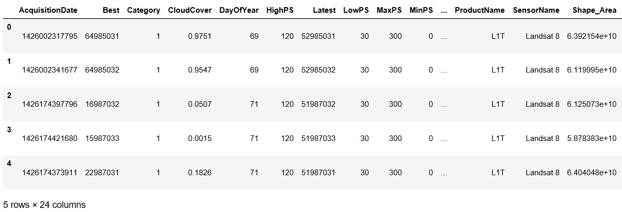

In order to verify this, I can check and see how many footprints were returned.

print("There are " + str(len(image_service_sdf)) + " Landsat image service footprints over New Jersey.")

There are 535 Landsat image service footprints over New Jersey.

Viewing the Footprints in ArcGIS Online

Before I can convert the image service footprints to a feature class, I need to convert the AcquisitionDate from Unix time to a pandas datetime object; otherwise, the API for Python will throw an error. This can be done very easily with the pandas to_datetime method.

import pandas as pd
image_service_sdf['AcquisitionDate'] = pd.to_datetime(image_service_sdf['AcquisitionDate'] /1000,unit='s')

Now, I can verify the spatial filter worked by viewing the footprints to ArcGIS Online or viewing them in ArcMap. I will add them to ArcGIS Online using import_data.

item = gis.content.import_data(df=image_service_sdf) 

I will verify that the item now exists in portal as a Feature Layer.

item

I will also load the footprints onto the map to visualize them.

map2 = gis.map("New Jersey", zoomlevel = 6)
display(map2)
map2.add_layer(item, {"renderer":"None"})

Exporting Footprints to a Feature Class

The spatial dataframe can very easily be converted into a feature class using the to_featureclass method. I will save the image service footprints to a feature class named nj_landsat_footprints.

import os
footprint_fc =  r'C:\PROJECTS\STATE_OF_THE_DATA\DATA\usa_states\usa.gdb\nj_landsat_footprints'
image_service_sdf.to_featureclass(os.path.dirname(footprint_fc),
                                os.path.basename(footprint_fc),
                                overwrite='overwrite')

Performing Statistical Calculations on the Landsat Metadata

My motivation for doing this analysis is actually to demonstrate how easily I can use the spatial dataframe to perform statistical summaries of the imagery metadata. Having created a dataframe of only imagery metadata over New Jersey, I can now do statistical calculations that give us additional insight into our imagery data.

Collection Date

I am interested in how recently imagery over New Jersey was collected. I can use max to find the most recent image dates from my dataframe.

import datetime
most_recent_image_date = image_service_sdf['AcquisitionDate'].max()
print(most_recent_image_date)
#datetime.datetime.utcfromtimestamp(most_recent_image_date/1000).strftime('%Y-%m-%dT%H:%M:%SZ')

2017-07-14 15:40:05.235000

Similarly, I can use min to find the oldest image date in the dataframe.

mean_image_date = image_service_sdf['AcquisitionDate'].min()
print(mean_image_date)
#datetime.datetime.utcfromtimestamp(mean_image_date/1000).strftime('%Y-%m-%dT%H:%M:%SZ')

2013-08-20 15:41:30.238000

Cloud Cover

I can also analyze cloud cover in the Landsat scenes. What is the mean cloud cover of the scenes over New Jersey? How many scenes are there with zero cloud cover? These are questions that we can quickly answer using the spatial dataframe.

mean_cloud_cover = image_service_sdf['CloudCover'].mean()
print(mean_cloud_cover)

0.440778691589

The mean Cloud Cover is .4407.

I can also use the dataframe to find out how many scenes have fewer than 10% Cloud Cover.

pd.value_counts(image_service_sdf['CloudCover'].values<0.1, sort=False)

There are 131 scenes of the 535 (about 25% of scenes) that have less than 10% Cloud Cover.

Hopefully you can see the usefulness of using a spatial dataframe with image services. I’m just scratching the surface here. If you have any questions, let me know!

See Also

• Shotcharts Revisited - From NBA Stats to Feature Service in Less Than 20 Lines of Code
• St. Louis Imagery - 1990 to Now
• How to Create Pitch Charts with Python