How to Map the Infrared Universe with Astropy and ArcGIS

A guest post by Gregory Brunner

I love astronomy. In a previous life, I was fortunate to study astronomy and work with some of the coolest hyperspectral data collected by the Spitzer Space Telescope. So since joining Esri five years ago, I’ve had it on my mind to use ArcGIS to map the infrared universe using observations from Spitzer Space Telescope; observations with which I already have some familiarity.

Over the past few months I’ve been exploring the various Python packages that I could use for astronomy. Having not done anything with astronomy for the past eight years, I was very pleased to discover astropy and I immediately saw that there was potential for me to use astropy and arcpy to bring observations (i.e. images) from Spitzer Space Telescope into ArcMap. So I decided to devote some time to figuring out how to use astropy and arcpy to bring these images into ArcMap and work towards creating some spectacular maps of the nearby infrared universe.

It might not sound too practical to use ArcGIS to look at observations from a space telescope; however, I think that the image processing capabilities in ArcGIS could be really powerful tools to use to create a large scale map of the universe. So the idea I’m putting forth isn’t just to look at some nearby galaxies in ArcMap, but that using Python with ArcGIS, we could make some spectacular and interactive maps of the universe.

Composite of GLIMPSE I and II and MIPSGAL data of the Milky Way galactic plane

Astronomy from the Perspective of a Geographer

Back in my grad student days (2005 - 2008), SOAImage DS9 was the default viewer for astronomers and IDL was the most common programming language and environment. Images taken by CCDs on telescopes were generally delivered as FITS files and to my knowledge they still are. I’ve never seen FITS files used in GIS; however, I have noticed that GDAL does support reading FITS files. That being said, I have not been able to read a FITS file into ArcMap and would venture to say that the FITS file reader has not been implemented. For this blog post, I’m going to describe how I used astropy and arcpy to convert images of M51 (NGC 5194) from FITS files to TIFF files and how I manipulated the coordinates in order for the images to project in ArcMap as they would in DS9, or for that matter, on the sky.

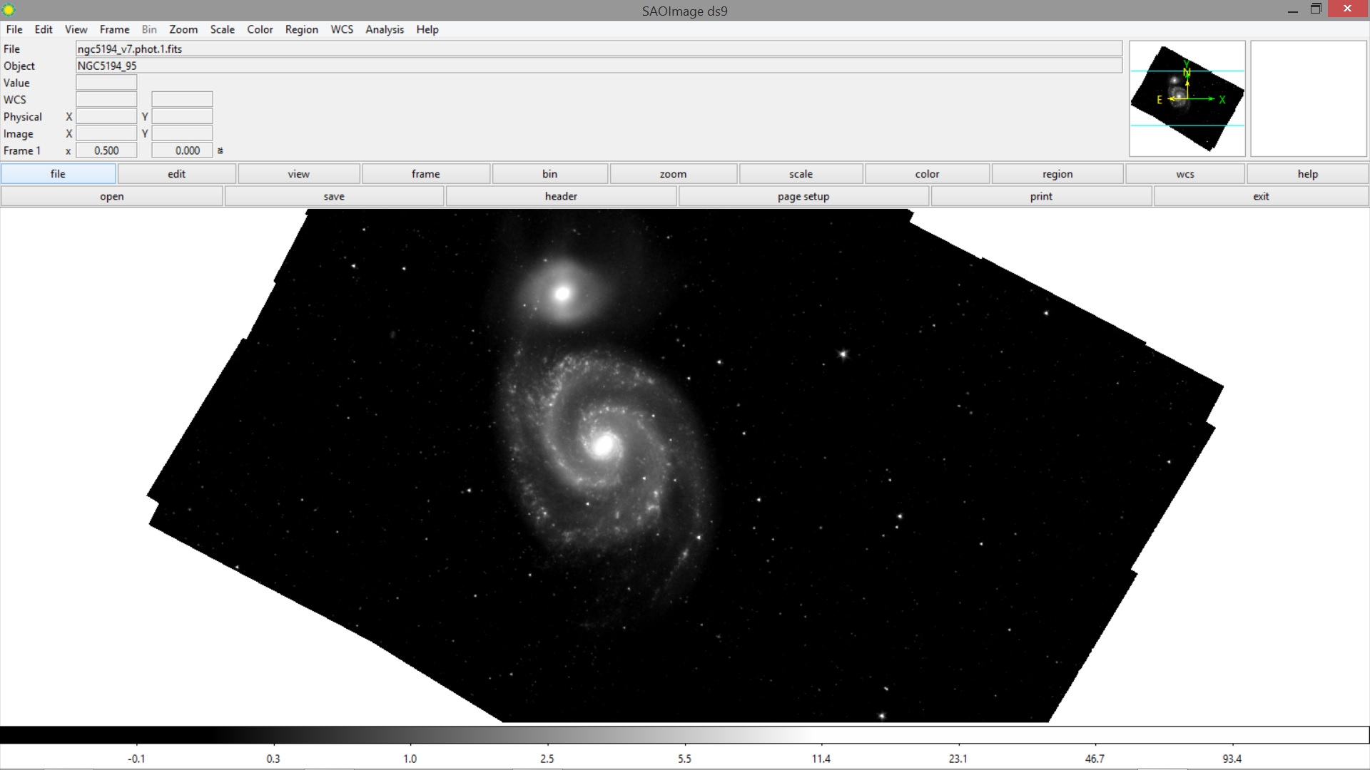NGC5194_Band1_DS9 Image of IRAC1 band of M51 in SAOImage DS9

In future posts, I plan to demonstrate how I batch downloaded these images from the Spitzer archive and how I mosaicked images from the GLIMPSE and MIPSGAL surveys into a map of the galactic plane. So if you find this post intriguing, come back soon to learn how to create more really beautiful maps of the sky.

The Data

I used the Spitzer Infrared Nearby Galaxies (SINGS) Infrared Array Camera (IRAC) data for M51. M51 is particularly striking when seen in the infrared, so I thought it would be a good galaxy to start with. I am also familiar with the observations.

I downloaded the four IRAC images. The numbers in the filename correspond to the band on the Infrared Array Camera. The wavelength corresponding to IRAC channels one through four are 3.6, 4.5, 5.8 and 8.0 microns respectively.

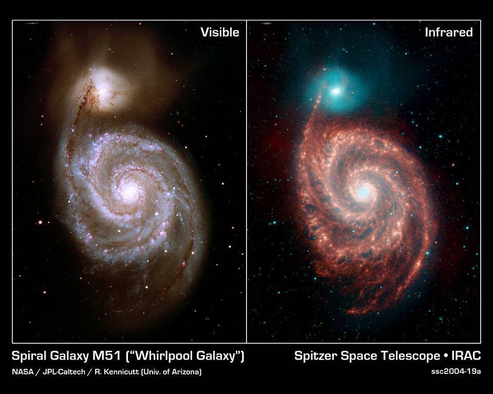M51 Image of M51 in the visible and infrared wavelength ranges

Imports and Environment Variables

To map the infrared universe, I needed to import numpy, astropy, sys, os, and arcpy. From astropy, I used the capability to handle FITS files and the utilities to work in the world coordinate system (WCS) projection. Here are my imports:

from __future__ import division

import numpy
from astropy import wcs
from astropy.io import fits
import sys
import os
import arcpy

I set some arcpy raster environment variables because I did not want to calculate pyramids or raster statistics. That’s something I don’t typically do, but I wasn’t happy with how the pyramids looked, so I opted to omit them knowing that I could always calculate them later.

arcpy.env.pyramid = "NONE"
arcpy.env.rasterStatistics  = "NONE"

Filenames

I knew I’d be reading and writing a bunch of image files. I had a folder that contained all of the input FITS files (input_image_path), a folder that I wrote the individual images out to as TIFFs (output_image_path), a folder where I wrote the four band composite images for a galaxy (composite_image_path), the number of bands (num_bands), and the instrument name (instrument). The galaxy name (galaxy) was also a variable. At the end of the post, I’ll show how I used a list of galaxies to loop through the 75 SINGS galaxies to make 4 band composite images of each of them. The composite image file (c_omposite_filename_ and composite_path_and_name) are both dependent on the galaxy name.

output_image_path = "C:/PROJECTS/R&D/ASTROARC/SINGS/TIFF/"
input_image_path = "C:/PROJECTS/R&D/ASTROARC/SINGS/FITS/"
composite_image_path = output_image_path + "COMPOSITES"
num_bands = 4
instrument = "IRAC"
galaxy = "ngc5194"
composite_filename = galaxy + "_" + instrument + "_" + str(num_bands) + "Bands.tif"
composite_path_and_name = os.path.join(composite_image_path, composite_filename)

I also had a few lines to check and make sure the output image folders exist before writing to them.

if not os.path.exists(output_image_path):
    os.mkdir(output_image_path)

if not os.path.exists(composite_image_path):
    os.mkdir(composite_image_path)

For Galaxy NGC5194…

I needed to loop through all four bands, define the input FITS filename (input_filename), a temporary output filename (temp_filename), and a “georeferenced” output filename (output_filename). I also had to join the filenames to their folders.

for num in range(1,num_bands+1):
    input_filename = galaxy + "_v7.phot." + str(num)+ ".fits"
    temp_filename = input_filename[:-4] + 'rev.tif'
    output_filename = input_filename[:-4] + 'rev.WCS.tif'
    temp_file_and_path = os.path.join(output_image_path, temp_filename)
    output_file_and_path = os.path.join(output_image_path, output_filename)
    input_file_and_path = os.path.join(input_image_path, input_filename)

Bear in mind as you read this, everything is being done within this for loop until I composite the bands.

Reading FITS File with Astropy

For each image file, I opened the file header and image data.

hdulist = fits.open(input_file_and_path)
w = wcs.WCS(hdulist[0].header)
image = hdulist[0].data

I used the image shape to define the pixel coordinates I’d use to reference the image. I needed the data as a numpy array to get the WCS coordinates and a string to pass to the Warp tool. I used the pixel coordinates to get the world coordinates at those points too.

pixcrd = numpy.array([[0, 0], [0, image.shape[0]],[image.shape[1], 0],
            [image.shape[1], image.shape[0]]], numpy.float_)
#Convert to string
pixcrd_string = '0 0;' + '0 ' + str(image.shape[0]) + ';' + 
            str(image.shape[1]) + ' 0;' + 
            str(image.shape[1]) + ' ' + str(image.shape[0])

# Convert pixel coordinates to world coordinates
world = w.wcs_pix2world(pixcrd, 1)
#Convert to string to project/warp in arcpy
coordinate_string = str(-1*world[0,0]) + ' ' + str(world[0,1]) + ';' + 
            str(-1*world[1,0]) + ' ' + str(world[1,1]) + ';' + 
            str(-1*world[2,0]) + ' ' + str(world[2,1]) + ';' + 
            str(-1*world[3,0]) + ' ' + str(world[3,1])

# Convert the same coordinates back to pixel coordinates.
pixcrd2 = w.wcs_world2pix(world, 1)

These are the coordinates that I used to “project” the M51 images.

Converting to TIFF

I needed to write the images out as “georeferenced” TIFF files. I flipped the y-axis of the image, defined the pixel data type to be 64-bit floats, then wrote the raster to disk.

#Converting raster to TIFF image
assert numpy.max(numpy.abs(pixcrd - pixcrd2)) < 1e-6
#Reversing the array
flipim = numpy.flipud(image)
#Writing the array to a raster
double_image = numpy.float64(flipim)
myRaster = arcpy.NumPyArrayToRaster(double_image)
myRaster.save(temp_file_and_path)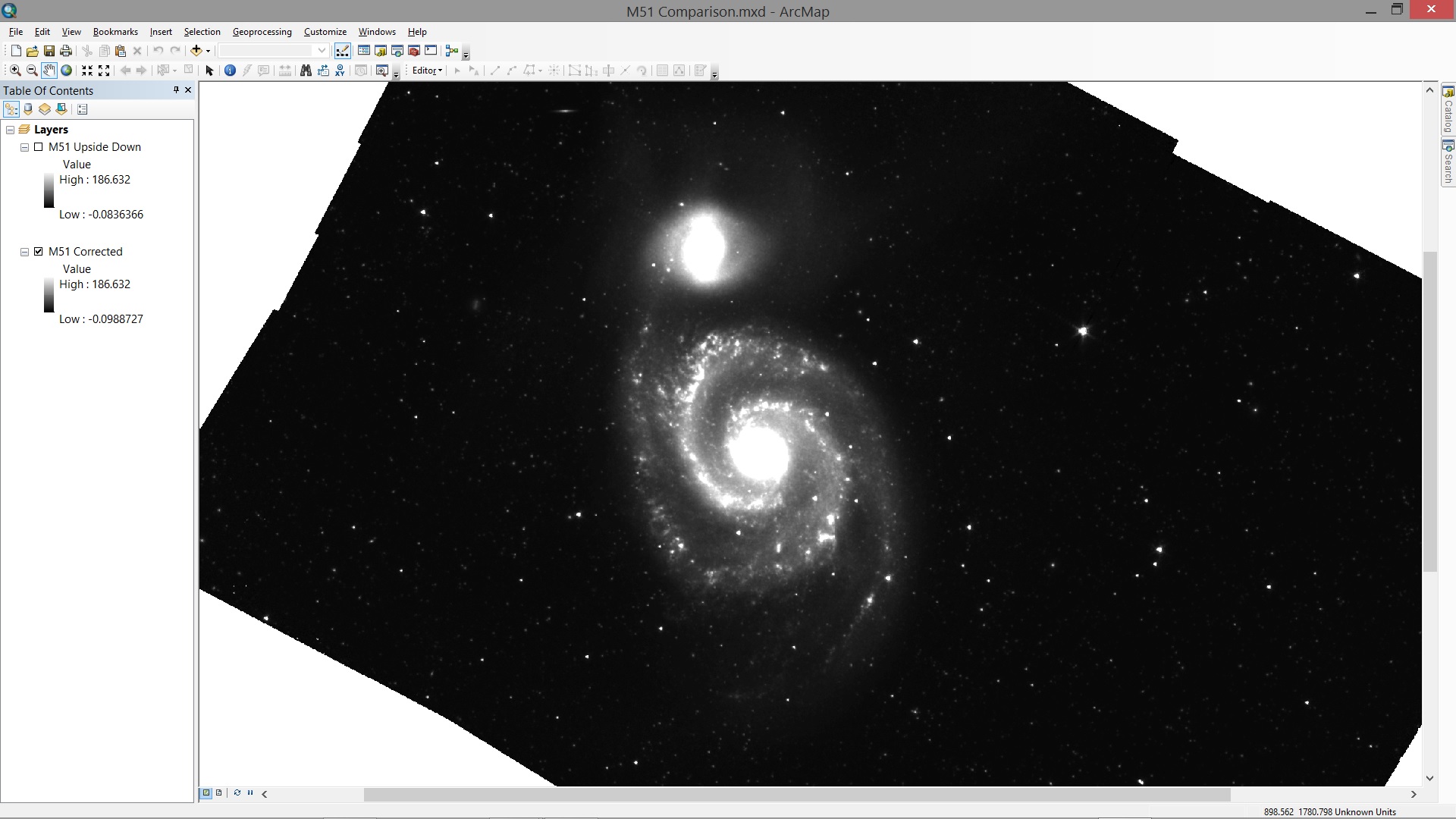

Here’s the IRAC1 image in ArcMap:

alt M51_IRAC1_rightside

If I didn’t flip the y-axis (numpy.flipup), the output image would have looked like:

alt M51_IRAC1_upside_down

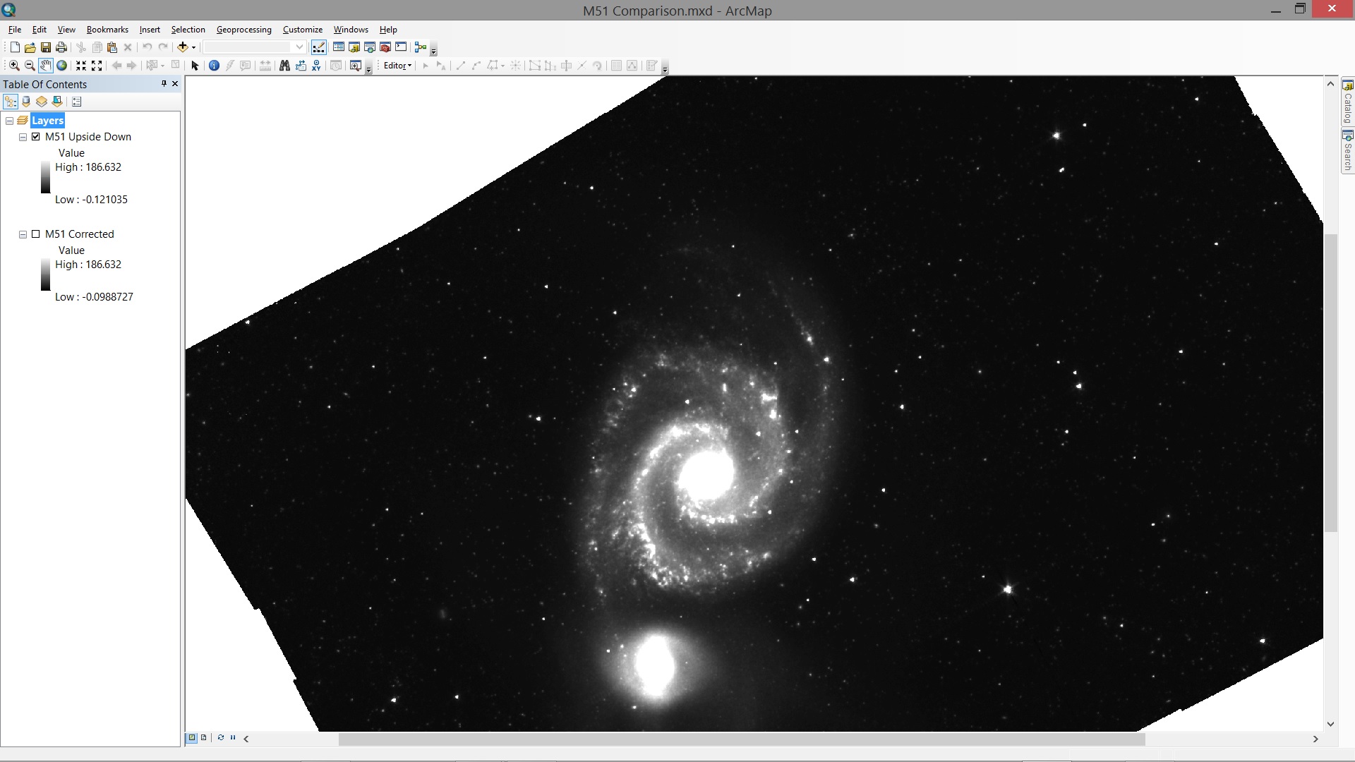
Finally, I Warped the image in order to give it WCS coordinates and deleted the temporary image (temp_file_and_path).

source_pnt = pixcrd_string
target_pnt = coordinate_string
arcpy.Warp_management(temp_file_and_path, source_pnt, target_pnt,
            output_file_and_path, "POLYORDER1","BILINEAR")
#Deleting the unreferenced image
arcpy.Delete_management(temp_file_and_path)

Composite Bands

I composited the four individual images into a single raster that has four bands.

arcpy.env.workspace = output_image_path
rasters = arcpy.ListRasters(galaxy + "*", "TIF")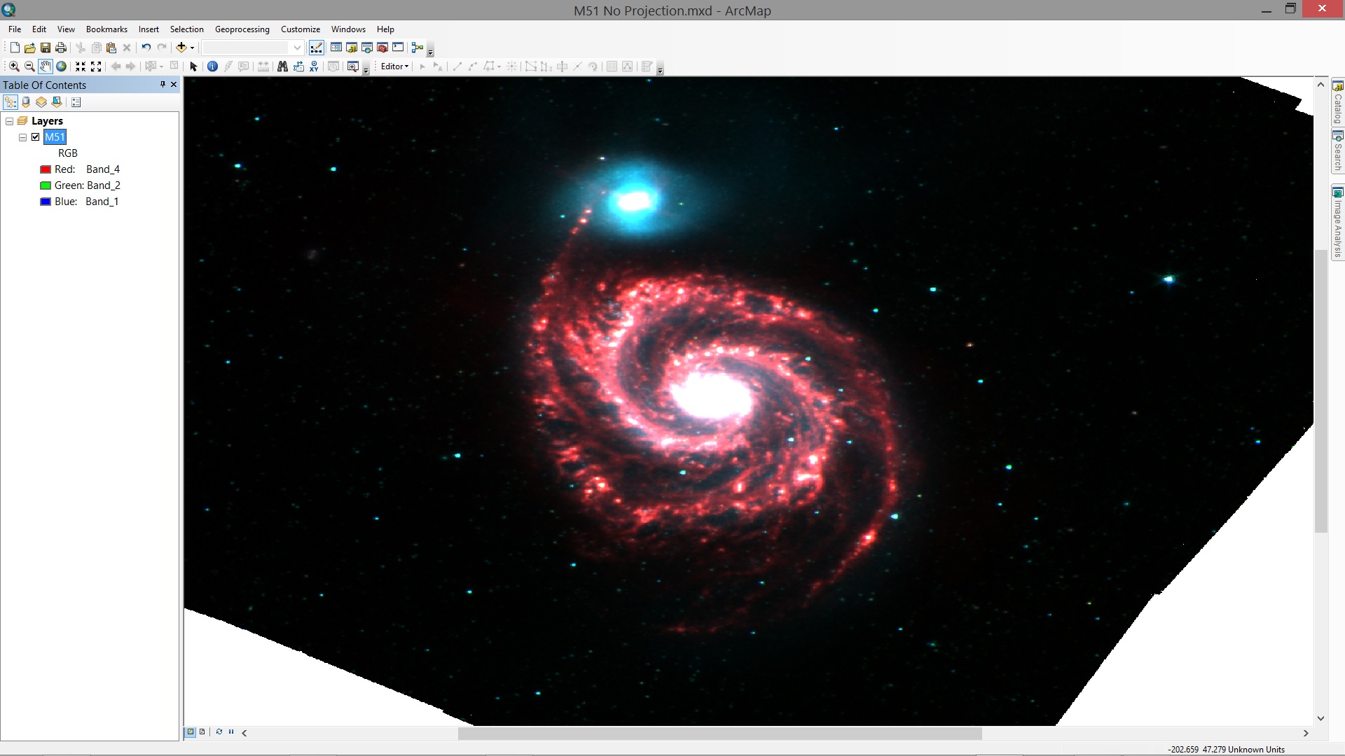
arcpy.CompositeBands_management(rasters,composite_path_and_name)

Note that this happened outside of the for loop (for band in num_bands).

I didn’t define the projection, so in ArcMap, M51 looked a little bit squished compared to the Spitzer image that I showed at the top.

M51_NoProjection

If I defined the projection to be WGS 1984, the image would look very similar to the image at the beginning of this post. I defined the projection when I added the galaxies into a single mosaic dataset.

Creating the Mosaic Dataset and Adding the Images

I then added the composite 4-band image into a mosaic dataset where I set image projection to be WGS 1984.

coordinate_sys = "PROJCS['WGS_1984_Web_Mercator_Auxiliary_Sphere',GEOGCS['GCS_WGS_1984',DATUM['D_WGS_1984',SPHEROID['WGS_1984',6378137.0,298.257223563]],PRIMEM['Greenwich',0.0],UNIT['Degree',0.0174532925199433]],PROJECTION['Mercator_Auxiliary_Sphere'],PARAMETER['False_Easting',0.0],PARAMETER['False_Northing',0.0],PARAMETER['Central_Meridian',0.0],PARAMETER['Standard_Parallel_1',0.0],PARAMETER['Auxiliary_Sphere_Type',0.0],UNIT['Meter',1.0]];-20037700 -30241100 10000;-100000 10000;-100000 10000;0.001;0.001;0.001;IsHighPrecision"
imagery_spatial_ref = "GEOGCS['GCS_WGS_1984',DATUM['D_WGS_1984',SPHEROID['WGS_1984',6378137.0,298.257223563]],PRIMEM['Greenwich',0.0],UNIT['Degree',0.0174532925199433]];-400 -400 1000000000;-100000 10000;-100000 10000;8.98315284119522E-09;0.001;0.001;IsHighPrecision"
mosaic_gdb = r"C:\PROJECTS\R&D\ASTROARC\SINGS\Spitzer.gdb"
mosaic_name = "SINGS"
mosaic_dataset = os.path.join(mosaic_gdb, mosaic_name)
arcpy.CreateMosaicDataset_management(mosaic_gdb, mosaic_name, coordinate_sys,
        num_bands="", pixel_type="", product_definition="NONE",
        product_band_definitions="")
arcpy.AddRastersToMosaicDataset_management(mosaic_dataset, "Raster Dataset",
        composite_image_path, "UPDATE_CELL_SIZES", "UPDATE_BOUNDARY",
        "NO_OVERVIEWS", "", "0", "1500", imagery_spatial_ref, "#", "SUBFOLDERS",
        "ALLOW_DUPLICATES", "NO_PYRAMIDS", "NO_STATISTICS",
        "NO_THUMBNAILS", "#", "NO_FORCE_SPATIAL_REFERENCE")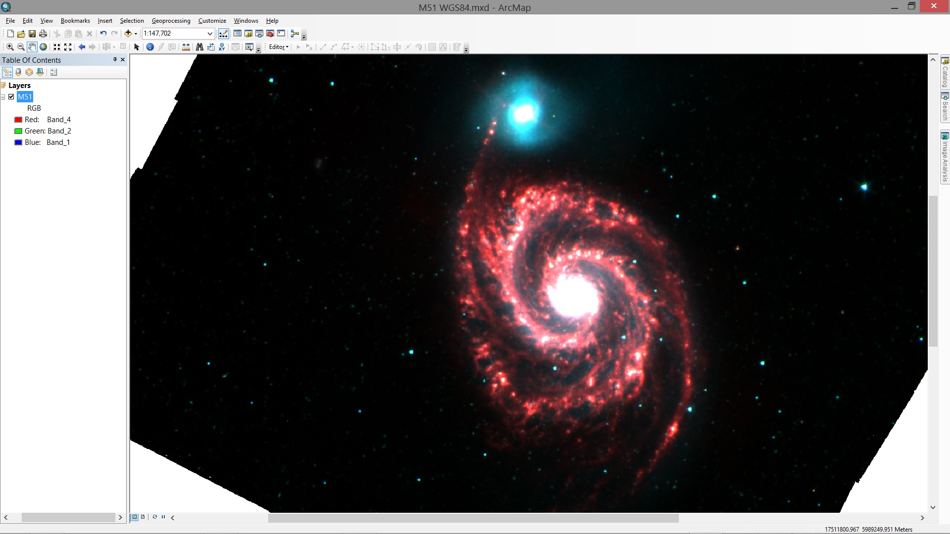

This should render the images very similarly to how you see it above in the NASA press release image. Here’s M51 in the mosaic dataset with the band combination set to use IRAC4 (red), IRAC2 (green), and IRAC1 (blue) as the band combination.

M51_WGS84_ArcMap

Mosaicking All 75 SINGS Galaxies

I structured the code so that I could do this for all 75 SINGS galaxies. In fact, I downloaded them all using the Python requests library and inserted a for loop where I defined the galaxy name and used the galaxy list as the input to the for loop.

galaxy_list = ['ngc0024', 'ngc0337', 'ngc0584', 'ngc0628', 'ngc0855', 'ngc0925',
            'ngc1097', 'ngc1266', 'ngc1291', 'ngc1316', 'ngc1377', 'ngc1404', 
            'ngc1482', 'ngc1512', 'ngc1566', 'ngc1705', 'ngc2403', 'ngc2798',
            'ngc2841', 'ngc2915', 'ngc2976', 'ngc3049', 'ngc3031', 'ngc3034',
            'ngc3190', 'ngc3184', 'ngc3198', 'ngc3265', 'ngc3351', 'ngc3521',
            'ngc3621', 'ngc3627', 'ngc3773', 'ngc3938', 'ngc4125', 'ngc4236',
            'ngc4254', 'ngc4321', 'ngc4450', 'ngc4536', 'ngc4552', 'ngc4559',
            'ngc4569', 'ngc4579', 'ngc4594', 'ngc4625', 'ngc4631', 'ngc4725',
            'ngc4736', 'ngc4826', 'ngc5033', 'ngc5055', 'ngc5194', 'ngc5195',
            'ngc5408', 'ngc5474', 'ngc5713', 'ngc5866', 'ngc6822', 'ngc6946', 
            'ngc7331', 'ngc7552', 'ngc7793','ic2574', 'ic4710', 'mrk33', 'hoii', 
            'm81dwa', 'ddo053', 'hoi', 'hoix', 'm81dwb', 'ddo154', 'ddo165', 'tol89']   

for galaxy in galaxy_list:
    #Do everything I described above!

In the end, I had 75 4-band composite images in a single a mosaic dataset. I shared them as an image service and put them in this storymap:

Go to Storymap

I’m only highlighting 12 galaxies here, but if you want to see them all, go to this webmap and search around the image service table.

Still to Come…

I got really into this when I worked on it last summer but the code isn’t too clean. I thought about making a Python class for every Spitzer Legacy Program I wanted to look at, but I didn’t get too far with it. My code is on github. I think I’m going to devote another post to show how I created some beautiful maps of the galactic plane from the MIPSGAL and GLIMPSE surveys (like the one at the beginning of the post and this one below).

View larger map

In that post I’ll go through how I scraped the MIPSGAL and GLIMPSE archives with BeautifulSoup and requests. Let me know if you thought this was interesting! I’d love to build a more complete map of the sky and even think about how to do things like crowdsource the sky with other observations of space, so if this topic interests you or if you have links to other people who are doing something similar, please let me know!

How to Map the Infrared Universe with Astropy and ArcGIS

Subscribe

See Also